From Models to Dynamics: Physical Inference in AI

This is a blog form of the invited talk I gave at the Theoretical Physics for AI conference in January 2026. It was held at the Aspen Center for Physics.

Modern AI inference is implemented as long sequences of arithmetic operations. Whether we build a small multilayer perceptron or a large transformer, our models are algebraic machinesI’ll refer to “arithmetic” and “algebraic operations” interchangeably. : inference consists of executing a long, ordered sequence of discrete mathematical operations. Across architectures, the list of primitives is remarkably small: matrix vector multiplies, nonlinearities, and occasional normalization steps. In practice, modern ML frameworks like Tensorflow, PyTorch, and JAX compile model descriptions into computational graphsOr in the case of JAX, an intermediate representation serving a similar role. that explicitly specify the ordered sequence of arithmetic operations required for inference.⊕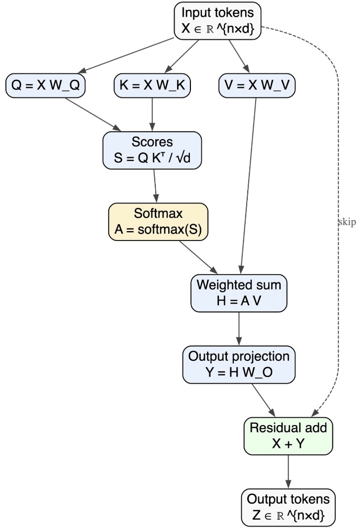

Why does inference take this form?

These computational structures are extremely efficient on today’s digital hardware. Certain operations—most notably dense linear algebra—map well onto GPUs and other accelerators. More fundamentally, digital computation favors a particular style of model formulation. Digital processors based on the von Neumann architecture execute programs via a strict fetch-decode-execute cycle: instructions and data are loaded from memory, an operation is performed, and the result is written back to registers or memory. This execution model is ideally suited to performing algebra step by step.

It is therefore natural—perhaps inevitable—that our first attempts at building intelligence express it as sequences of discrete algebraic operations. But this formulation does not appear to be a fundamental requirement of intelligence. Rather, it is the result of optimizing our models to fit the constraints and affordances of digital hardware. Inference-as-algebra reflects the execution model of our hardware, not a necessity imposed by intelligence itself.No form of biological intelligence seems to be performing arithmetic in the way that GPUs are.

In the long arc of artificial intelligence, we are still at the beginning. There will be many ways to build intelligence, and many of them will not be arithmetic.

As we scale models, we run into latency, energy, and bandwidth limits. And so we may ask ourselves: rather than simulating AI inference as arithmetic, can we build physical systems that embody inference directly? In other words, can we take the computation of today’s AI inference and embody it in physics, rather than simulate it with arithmetic?

Inference on an energy landscape

One way to think about modern AI inference—without framing it as a long sequence of algebraic operations—is as dynamics on an energy landscape. An energy-based model (EBM) assigns to every possible stateHere, a state refers to a high-dimensional configuration of the model, such as a token embedding, a latent vector, or the pixel values of an image. $x$ a scalar energy $E(x)$. Intuitively, lower-energy states correspond to configurations that are more consistent with the data, while higher-energy states are less so.Much of generative modeling can be viewed as learning an approximation to the underlying high-dimensional probability distribution of the world—for example, the distribution governing natural language or images. . This intuition is commonly formalized by defining a probability distribution over states via the Boltzmann distribution

where $Z$ is the partition function that ensures proper normalization.Computing the partition function is generally intractable, as it requires integrating over an enormous, often effectively uncountable, state space. For domains like natural language, exact evaluation would require enumerating all possible sentences. In practice, this motivates working directly with energies rather than normalized probabilities. In this view, learning corresponds to shaping the energy landscape so that data-consistent states lie in low-energy regions, while inference corresponds to sampling from those low-energy configurations.

Crucially, EBMs do not intrinsically prescribe inference as a discrete sequence of algebraic steps. Instead, inference can be formulated as a dynamical process: the state evolves over time so as to move from regions of higher to lower energy, eventually settling into a locally stable configuration of the energy landscape.

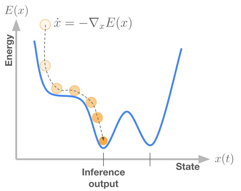
A useful analogy is that of a ball rolling downhill until it comes to rest. Formally, this “rolling downhill” behavior can be expressed as gradient flow dynamics

which are run until the system relaxes to a stationary point where the velocity vanishes.I will use the terms “attractor states”, “fixed points”, and “stationary points” interchangeably to denote local minima of the energy function. Stable fixed points of the dynamics, typically local minima of $E(x)$, correspond to inference results or model outputs. In this view, time itself is the axis of computation.

In this formulation, computation is not carried out instruction by instruction. Instead, inference emerges from the continuous-time relaxation of a mathematical—and potentially physical—system toward relaxation. This view of inference is fundamentally different from the von Neumann execution model: computation is performed by the evolution of state under fixed dynamics, rather than by executing a prescribed sequence of instructions.

Dense Associative Memory: a canonical energy-based model

Many modern models that are usually written as iterative algorithms can be re-expressed as gradient flow on an energy function. Dense Associative Memory (DenseAM) provides a minimal, circuit-level realization of this idea through a model that is simple in structure yet surprisingly expressive.

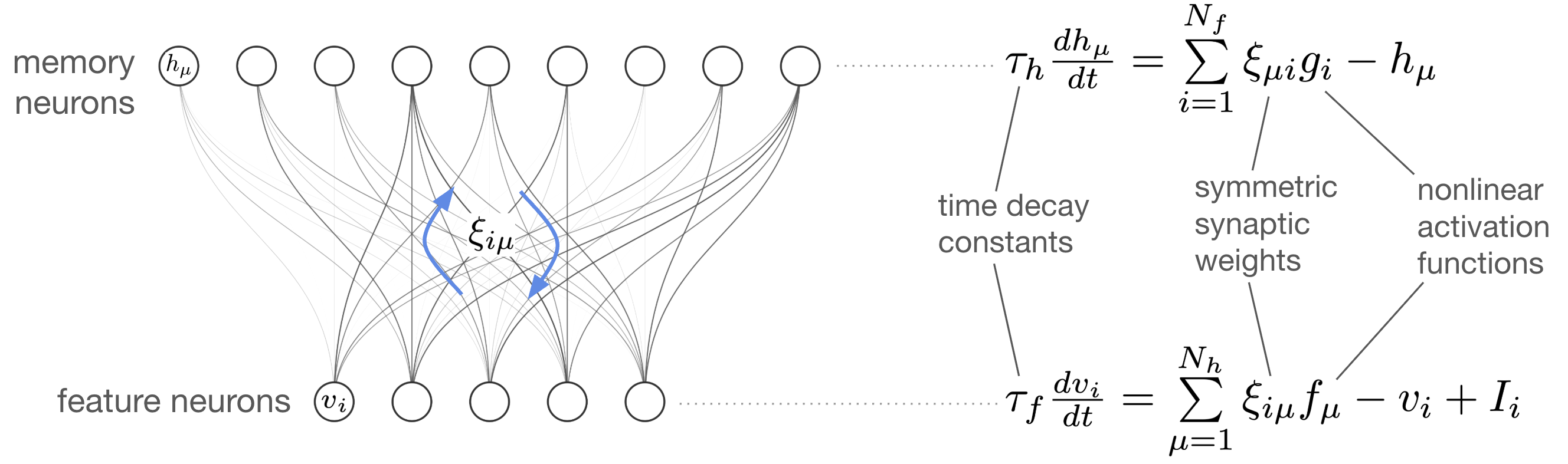
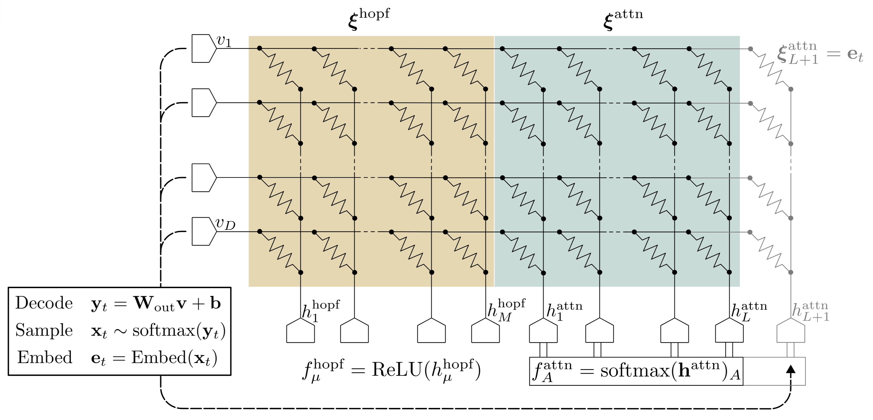
A DenseAM can be formulated as a bipartite system consisting of feature (visible) neurons and memory (hidden) neurons, coupled through a weight matrix $\boldsymbol \xi$. The evolution of the neuron states is governed by coupled differential equations (shown on the right of the schematic). Because DenseAM is an energy-based model, these dynamics are exactly the gradient flow dynamics of an implicit energy function $E(v, h)$. In other words, the system evolves so as to monotonically decrease its energy until it reaches a stable stationary point.This is exactly the idea of a Lyapunov energy function in dynamical systems theory. When a Lyapunov energy exists for a system, this means that the system has stable attractor states. Energy functions are a powerful tool for analyzing the behavior of dynamical systems.

What makes DenseAM remarkable is that, with different activation functions $g$ and $f$, the same underlying dynamical system can realize behaviors typically associated with very different model classes, ranging from attention mechanisms and transformer-style inference to diffusion-like dynamics.

Crucially, this does not mean that DenseAM shares the computational structure of transformers or diffusion models.For example, you won’t be able to take a pre-trained transformer model and just plug it into your DenseAM. The weight matrices and parameterization of the models are totally different. Those models are prescribed as feedforward or iterative update rules, while DenseAM computes the same functions implicitly as the fixed points of its continuous-time dynamics. What appears as feedforward computation in a digital model is realized here as the endpoint of physical relaxation on an energy landscape.

Gradient flow as a physical process

So far we’ve seen how dynamical systems can serve as a different primitive of computation. Rather than executing long sequences of algebraic operations, complex functions can be realized as the fixed points of continuous-time dynamics. In this view, models like transformers are not fundamentally defined by their arithmetic structure, but by the equilibria of a dynamical system.

⊕In both roles, energy is a mathematical construct, rather than a literal physical quantity. It is never directly stored, measured, or dissipated as physical energy. Instead, it is a tool to characterize the behavior of a class of dynamical systems: specifically those systems that realize fixed point attractors. The same idea of energy minimization that defines the inference process is the tool used to study the dynamical systems that exactly implement that inference process. At the core, linking these two ideas, is the idea of energy: first as a quantity related to the probability distributions our models learn, and secondly as a tool to describe a class of dynamical systems (specifically the class of dynamics that realize fixed-point maps). Energy is the abstract link between model and hardware, between algorithm and computation.

Dynamical systems are found in the world all around usDifferential equations are the natural tool for describing systems that are continuous in time and continuous in state, two defining properties of analog systems. . Many naturally occurring systems evolve according to differential equations that can be written as gradient flow on some Lyapunov energy functionA wide class of stable systems admit Lyapunov energy functions. When such a function exists, the system is guaranteed to relax toward attractor states. . This observation suggests a natural alternative to algebraic computation: rather than simulating energy descent digitally, one can build a physical system whose intrinsic dynamics already perform it.

This is the key conceptual shift: Inference, when cast as gradient flow, is a physical process. Computation occurs through the time evolution of this physical process, and useful inference is performed when the system’s dynamics match the gradient-flow dynamics of the target energy-based model. In this framing, hardware is no longer a substrate that executes an algorithm. Instead, it is the algorithm.

A physical energy-based model: electronic circuits for DenseAM

Electronics provides a rich toolkit for constructing a wide class of dynamical systems. In our recent work, we built a physical realization of DenseAM by translating its system of coupled differential equations into a single, large-scale analog circuit design that obeys the same equations of motion.

⊕The details of the circuit implementation will have to wait for a separate blog post. Here, I’ll focus on the conceptual implications rather than implementation details.

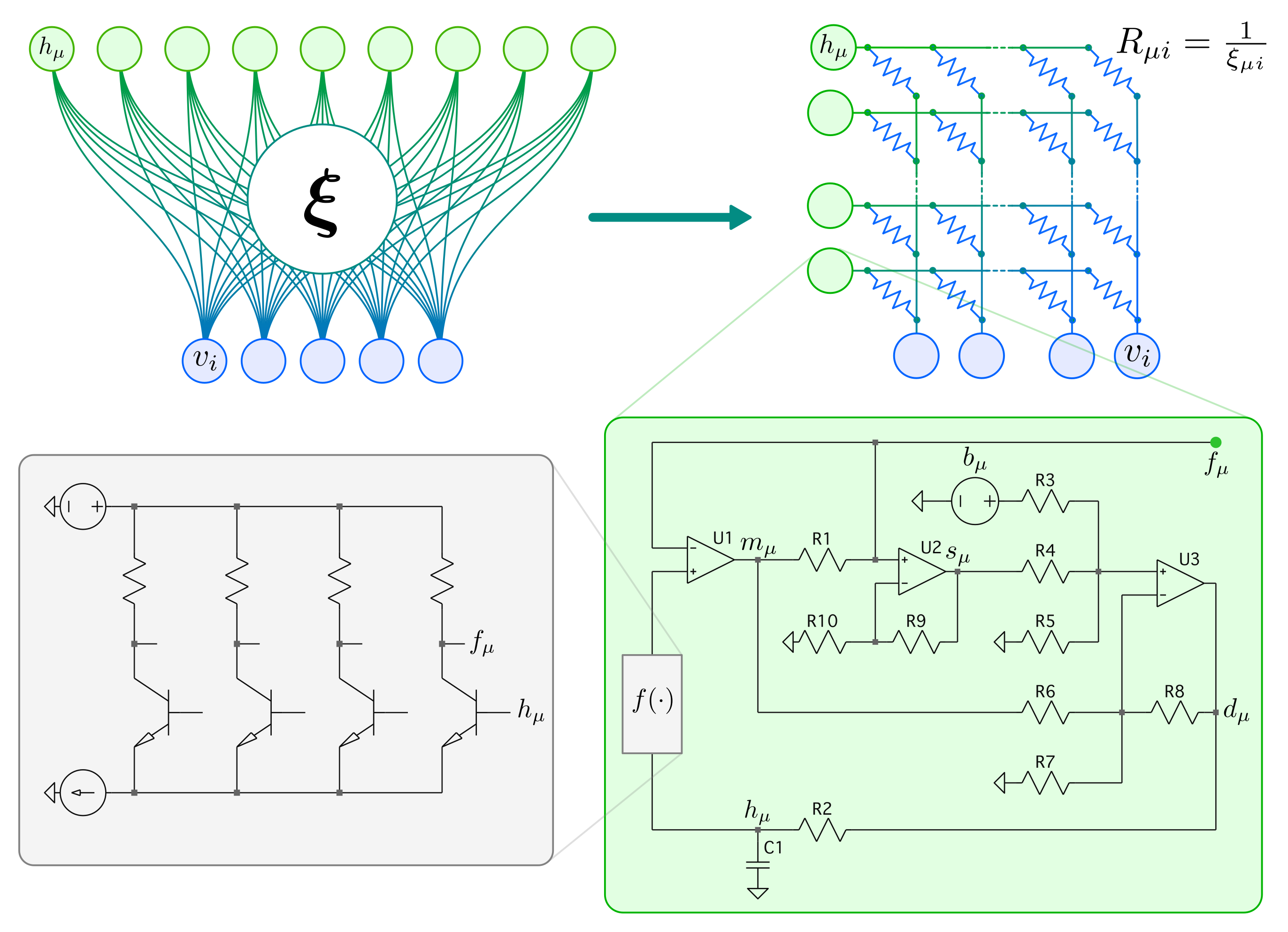
In this design, the model’s dynamics and the hardware’s physics are the same object. Analog electronic components (resistors, capacitors, amplifiers) naturally implement the operations required by the DenseAM equations. Model states are represented as voltages, synaptic weights as resistances, and the interactions between states and weights generate currents that drive the time evolution. The resulting circuit obeys the same coupled differential equations as the abstract model. Computation is no longer an algorithm like an ODE solver; it is the system evolving in time.

This highlights a key distinction between this class of hardware and the digital processors used for modern AI:

Digital processors simulate inference step-by-step.

Physical systems obey them.

In digital hardware, gradient flow is approximated through a sequence of arithmetic operations executed under a clock. In contrast, in an analog circuit, gradient flow is the natural behavior of the system itself.

Inference time is set by physics, not model size

By now, it may feel intuitive to use physical systems to realize inference dynamics directly, rather than simulating them step by step on digital processors. That intuition turns out to be correct, and it has a striking conseequence for inference latency.

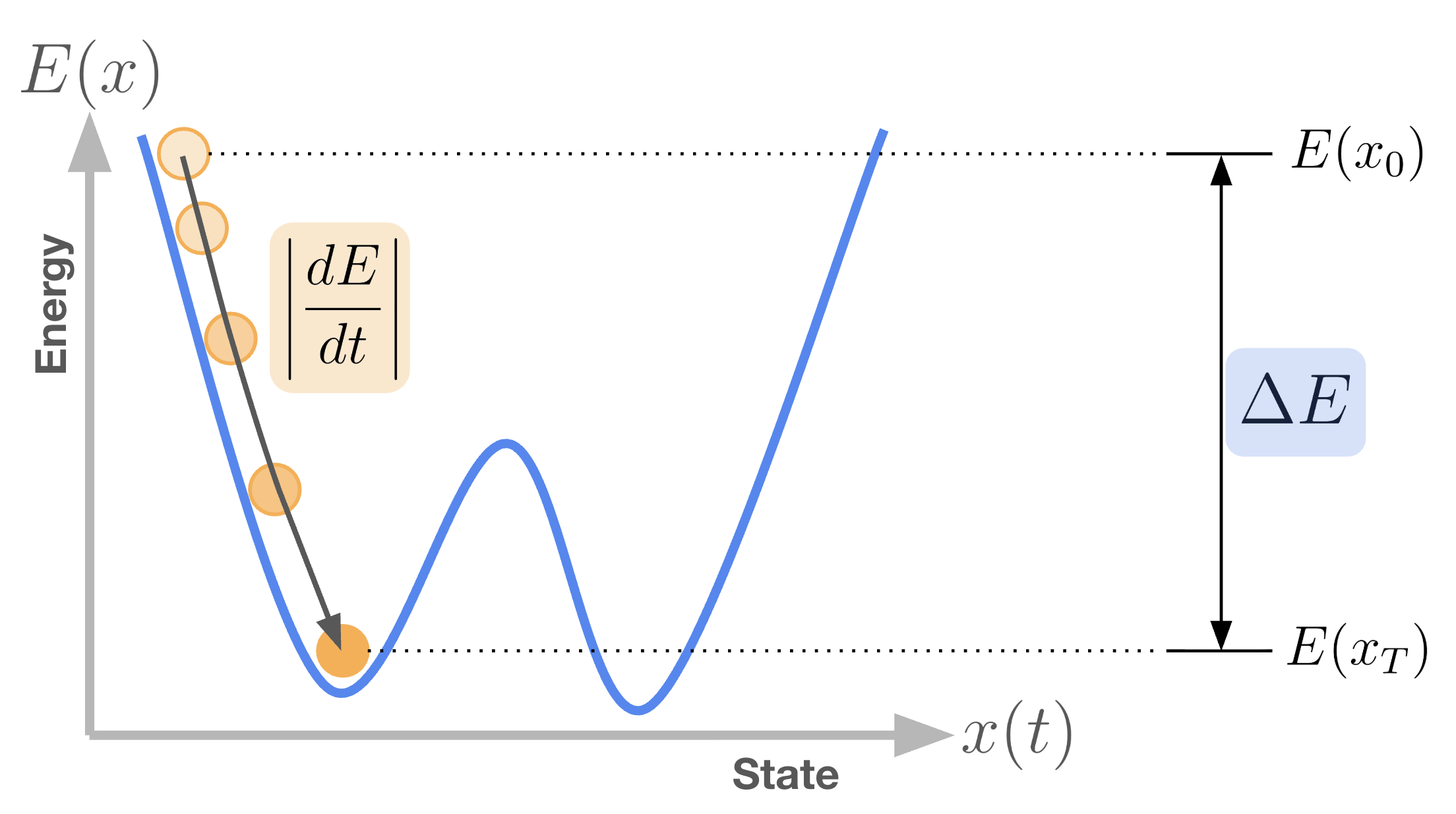
Recall that the energy function used to analyze these dynamics is a mathematical construct, introduced because it is useful for understanding system behavior. In particular, it allows us to reason about how long inference takes. Uisng the familiar analog of a ball rolling downhill, we can characterize inference by two quantities:

• the total energy drop $\Delta E$ between the initial state and the final attractor, and
• the rate at which energy decreases along the trajectory, $\frac{dE}{dt}$.

⊕This should not be read as an exact formula, but as a scaling argument and an intuition. For rigorous proof of the convergence time claim, please refer to Appendix E of our paper. Heuristically, the convergence timeFrom here on, I will refer to convergence time and inference time as the same thing, because when the system converges is when inference is complete. can be estimate as

The key result is that, for DenseAM, both $\Delta E$ and $\vert dE/dt\vert$ scale in the same way as the model size increases. As the number of neurons and weights grows, the energy landscape becomes higher dimensional, but its characteristic depth and curvature scale proportionally. As a result, the slowest relaxation mode of the system remains unchanged. Consequently, inference time remains constant with respect to model size: $T_\text{conv}\sim\mathcal O(1)$.

This behavior stands in sharp contrast to digital systems, where inference latency scales with the number of arithmetic operations performed. In continuous-time systems, inference ends when the system relaxes to equilibrium. That relaxation time is governed by device-level time constants, not by the number of neurons, layers, or parameters.

Transformer-like models with constant-time inference

⊕Because EBMs are guaranteed to converge to fixed points, their final state of inference is robust in the sense that neuron values are not moving anymore. This makes their inference robust to a variety of imperfections in the analog world, and removes the requirement that neuron values be read out simultaneously. As discussed earlier, DenseAM is compelling because it can express a wide range of modern AI models, including attention mechanisms and transformer-like architectures, all within a single dynamical framework. In this section, we adopt the formulation proposed in Energy Transformer to construct a transformer-like model using DenseAM as the underlying primitive.

The key idea is not that DenseAM implements a transformer in the conventional architectural sense, but that it realizes the same input-output map as a transformer block, expressed instead as the fixed point of an energy-based dynamical system. This formulation is especially appealing because it admits a direct analog circuit realization, rather than requiring digital simulation.

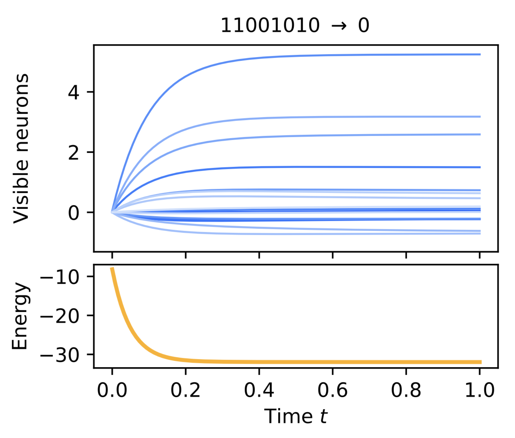
Concretely, we trained an Energy Transformer on a bit-string parity task.In our experiments, training was performed digitally (on GPU) using automatic differentiation through an ODE solver. Inference proceeds by programming the dynamic weights of the energy attention DenseAM and allowing the system to evolve according to its continuous-time dynamics until it reaches a steady state. The final values of the visible neurons are then read out, decoded, and sampled to produce the next token.

Structurally, the Energy Transformer consists of two coupled DenseAM systems. First, a DenseAM equivalent to a modern Hopfield network plays the role typically occupied by the feedforward network within a transformer block. Second, a separate DenseAM with a softmax activation on the hidden neurons realizes the energy function associated with attention.

Coupled together, the joint gradient-flow dynamics of these two DenseAMs reproduce the behavior of a standard transformer block, with a crucial distinction: depth is replaced by time. Rather than applying attention and feedforward layers sequentially, inference emerges as the relaxation of a single high-dimensional dynamical system.

Autoregressive inference proceeds by repeatedly:

1. Allowing the visible neurons to relax until convergence
2. Decoding and sampling the next token from the visible neuron state
3. Re-embedding that token and adding it to the attention DenseAM

The weights of the Hopfield DenseAM $\boldsymbol\xi^\text{hopf}$ are fixed, while the weights of the attention DenseAM $\boldsymbol\xi^\text{attn}$ depend on the context tokens. When a new token is generated, it is added to the context by appending its embedding vector to $\boldsymbol\xi^\text{attn}$.

Each autoregressive inference step increases the dimensionality of the system by introducing a new degree of freedom, yet the time required for the system to relax remains $\mathcal O(1)$. Inference latency is governed by the physical time constants of the system, not by context length or model width.

Estimates of inference time with existing hardware

If inference latency depends not on model size but on physics, how fast can it be?Of course, we do not claim that a hardware implementation can be scaled arbitrarily. Depending on the hardware (process node, design choices, power constraints, etc.), there will be a point at which a fabricated circuit no longer accurately represents the intended DenseAM dynamics. Beyond that point, our inference-time scaling claims no longer apply—but neither do claims that the system is implementing a DenseAM in the first place. As discussed above, convergence time is set by two quantities: the energy gap $\Delta E$ to be traversed, and the rate at which energy decreases along the gradient-flow trajectory, $\frac{dE}{dt}$. Because the dynamics follow gradient flow, decreasing the time constants of the system directly increases $|dE/dt|$, thereby accelerating convergence.

but because the dynamics are gradient flow, $\tau_v\frac{dv_i}{dt}=-\frac{dE}{dv_i}$ and ${\tau_h\frac{dh_\mu}{dt}=-\frac{dE}{dh_\mu}}$. So, $\frac{dE}{dt}$ is proportional to $1/\tau_v$ and $1/\tau_h$, and so $\frac{dE}{dt}$ grows when the time constants shrink.

However, the time constants of the dynamics cannot be made infinitely small. Our circuit realization relies on amplifiers, whose bandwidth and large-signal response impose fundamental limits on how fast the system can evolve.Passive components in our design (resistors, capacitors, triode-regime transistors) do not impose speed limits.

A standard amplifier model captures two key constraints:

• Slew rate (SR). The slew rate limits the maximum rate of change of the output voltage, i.e. $\left\vert\frac{dV_\text{out}}{dt}\right\vert\le\text{SR}$. If the system dynamics demand faster voltage change than the amplifier can provide, the dynamics become slew-limited and slow down accordingly.
• Gain-bandwidth product (GBW). The gain-bandwidth product limits the small-signal bandwidth of the amplifier. For a closed-loop gain $A_\text{cl}$, the effective bandwidth is approximately $f_\text{BW}\approx\frac{\text{GBW}}{A_\text{cl}}$, which imposes a lower bound on achievable time constants of $\tau\gtrsim\frac{1}{2\pi f_\text{BW}}$.

Given constraints from both SR and GBW, the minimum achievable time constant of the system can be conservatively estimated as roughly one order of magnitude larger than the most restrictive of these limits. Furthermore, taking convergence to require on the order of 10 time constants,a standard engineering heuristic for exponential relaxation, which fits our model we can estimate total inference latency. With this model, we can plot the expected convergence time as a function of amplifier slew rate and gain-bandwidth ratio.

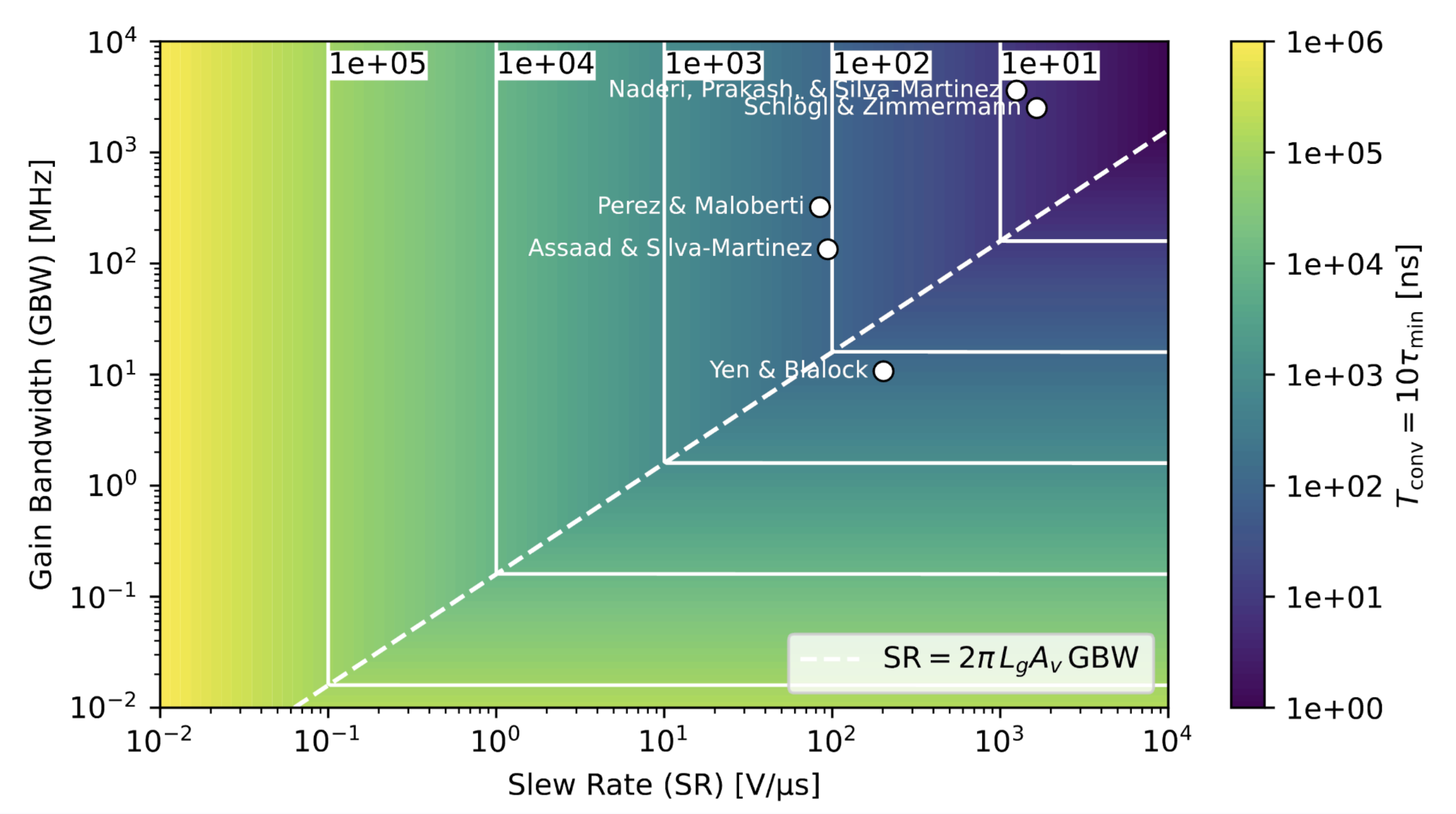
In the upper right corner of the plot, convergence times fall in the nanosecond regime and are achievable with existing amplifier designs reported in the literature. Crucially, these inference time estimates are independent of model size. They do not scale with the number of neurons, the number of parameters, or the context length.

Inference latency is set by device physics, not by arithmetic count.

Towards inference as physical dynamics

What I hope to have shown is a different way of thinking about AI inference.

In the dominant paradigm today, inference is treated as the execution of algebra: a long sequence of discrete arithmetic operations. This view has been shaped by the constraints of digital hardware, and it has served us extraordinarily well. But it is not the only way to compute, nor does it appear to be a fundamental description of intelligence.

Energy-based models offer an alternative formulation. In EBMs, inference is described as the evolution of a state under a dynamical system towards equilibrium. When such dynamics admit a Lyapunov energy, inference can be understood as gradient flow on an energy landscape, and model outputs correspond to stable fixed points of that flow.

The EBM formulation opens the door to physical realization. If inference is defined by differential equations, then any physical system that obeys the same equations performs the same computation. These systems do not simulate inference like digital processors; they instantiate it.

Dense Associative Memory provides a concrete example of this idea. It is an expressive EBM whose dynamics can be mapped directly onto analog electronic circuits. When extended to energy-based attention mechanisms, it can realize transformer-like models while retaining inference set by device physics, not model size or context length.

This perspective suggests a broader shift. Inference has long been treated as arithmetic because that is what our hardware makes easy. When inference is formulated as dynamics, computation becomes a property of physical systems themselves.

As AI models increasingly look like physical systems, the next step may be to let physics itself perform the computation.

Thanks for reading! If you enjoyed this, you might like taking a deeper dive into the details in our paper, Dense Associative Memories with Analog Circuits.