Quantization-Aware Training with Custom Gradients

The principle of hardware-aware training and quantization-aware training is that during the forward pass, the network uses the actual hardware, while in the backwards pass, the full precision weights are updated. The result is that backprop is able to learn the weights that best suit the actual hardware, because the error of the hardware is propagated through computing the derivatives.

I want to demonstrate two plausible-looking approaches to implementing quantization-aware training that actually have very different behaviors. We’re going to simulate this using custom gradients in Tensorflow. The actual quantize(...) method’s implementation is not particularly relevant, it’s simply a stand in for some lossy/noisy method of representing weights or inputs on hardware. Pay attention to where @tf.custom_gradient is used.

Approach 1: Custom gradient for quantization

With this approach, we define the custom gradient on the quantize function to simply pass the original gradient through. This is often referred to as a straight-through estimator. This makes sense because even though the quantize method rounds values off to a certain set of points, the direction of descent is still roughly the same as if the points were in one dimension. Autodiff will differentiate the matrix multiplication in quantized_layer and use the grad(dy) function defined inside quantize(...).

def round_to_nearest(x, level_values):
		...

@tf.custom_gradient
def quantize(inputs, n_levels):
    inputs_clipped = tf.clip_by_value(inputs, -1.0, 1.0)
    quantized_levels = tf.linspace(-1.0, 1.0, n_levels)
    inputs_quantized = round_to_nearest(inputs_clipped, quantized_levels)

    def grad(dy):
        return dy, None  # Straight-through estimator

    return inputs_quantized, grad

def quantized_layer(inputs, weights, bias, n_levels):
    q_i = quantize(inputs, n_levels)
    q_w = quantize(weights, n_levels)
    q_b = quantize(bias, n_levels)
    output = tf.matmul(q_i, q_w) + q_b
    return output

Approach 2: Custom gradient for layer

With this approach, we define a custom gradient before the quantize function, such that autodifferentiation does not use the chain rule through the call to tf.matmul, but instead follows the defined custom gradient. This custom gradient simply implements the standard derivatives of a matrix multiply $z=W^Tx+b$ where $\nabla_Wz=x$, $\nabla_xz=W$.

def round_to_nearest(x, level_values):
		...

def quantize(inputs, n_levels):
    inputs_clipped = tf.clip_by_value(inputs, -1.0, 1.0)
    quantized_levels = tf.linspace(-1.0, 1.0, n_levels)
    inputs_quantized = round_to_nearest(inputs_clipped, quantized_levels)

    return inputs_quantized

@tf.custom_gradient
def quantized_layer(inputs, weights, bias, n_levels):
    q_i = quantize(inputs, n_levels)
    q_w = quantize(weights, n_levels)
    q_b = quantize(bias, n_levels)
    output = tf.matmul(q_i, q_w) + q_b

    # this will stop the gradient computation from going into the custom gradient of quantize(...)
    def grad(dy, variables=None):
        # Gradients with respect to inputs
        grad_inputs = tf.matmul(dy, tf.transpose(weights))

        # Gradients with respect to weights
        grad_weights = tf.matmul(tf.transpose(inputs), dy)

        # Gradients with respect to bias
        grad_bias = tf.reduce_sum(dy, axis=0)
        return grad_inputs, grad_weights, grad_bias, 0

    return output, grad

Mathematical Comparison

These two approaches might seem at first glance like they do the same thing, but in fact they behave slightly differently. For simplicity let’s consider matrix multiplication without the bias term, which is defined for the original inputs as $z=W^Tx$. Then, the quantized version of this would be $z'=Q(W)^TQ(x)$, where $Q(…)$ is our quantization function. When we try to differentiate this, we see that computing $\frac{\partial z'}{\partial x}$ requires using the product rule:

Because we’re using the straight-through estimator for $Q(…)$, we say that $\frac{\partial}{\partial x}( Q(x))=1$. Further, since $\frac{\partial}{\partial x}(Q(W)^T))=0$, we can reduce to just the second term:

This is what Approach 1 implements, but is actually different than what’s implemented in the second code example, where the custom gradient is defined at the level of the layer. There, the gradient is computed as $\frac{\partial z’}{\partial x}=W^T$, using the original, unquantized weights.

From a mathematical perspective, approach 1 is correct, while approach 2 is not because it does not consider the effect of quantization.

Empirical Comparison

This difference in backprop implementation appears to play a significant role in the training dynamics. Here is the accuracy of a neural network with 50 hidden neurons, with weights and inputs quantized to 8 linear levels, on the KMNIST dataset downsampled to 20x20 images.

The dark green and dark red curves are the test set accuracies of the network with approach 1 (quantized gradient) and approach 2 (custom layer gradient), respectively. The lighter curves are the training set accuracies.

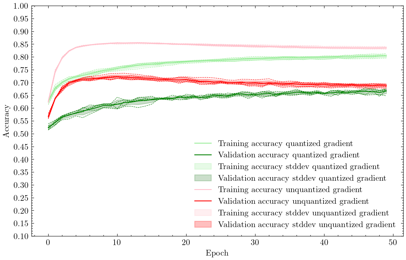
Interestingly, even though Approach 2 does not account for quantized weights and inputs during backprop, it results in much faster training. In just 5 epochs, the red curve reaches >70% accuracy, a figure that the network using Approach 1 never reaches even after 50 epochs of training. We also observe that backprop that ignores quantization seems to overfit, resulting in accuracy decreasing by a few percentage by the 50th epoch.

Both approaches seem to result in similar amounts of variability during training, with the shaded regions around the lines depicting one standard deviation of accuracy across 5 different runs. This is also a bit surprising, since one would expect backprop that ignores the effect of quantization to result in noisier training dynamics than backprop that includes the effect of quantization.