Toy Models of Analog Quantized Neural Networks

Here, I’m going to train a quantized multi-layer perceptron (MLP) with a single hidden layer on the KMNIST dataset downsampled to 7x7 images. With this toy model, I will investigate a few surprising phenomena, provide some explanations, and rediscover the behavior of weight oscillation during quantization-aware training.

Underparameterized Regimes

The goal is to explore the underparameterized regime of these neural networks, where the model doesn’t have the expressive power to fully do well on the problem. We get to this regime by moving along two axes:

1. Making the dataset harder, by downsampling KMNIST to 7x7 images
2. Making the network quite small (16 neurons in its hidden layer)

We won’t see any SOTA results on KMNIST classification accuracy, but that isn’t the point here. We’re going to focus on the change in behaviors between different approaches, with the goal of helping us make generalizable observations about larger NNs applied to more complex problems.

Analog Quantization

Digital quantization allows lots of tricks, including nonlinearly spaced levels and different quantization levels for different layers, but in analog neural network accelerators, this flexibility is not available. All weights and input activations can only be represented by a fixed set of levels that are determined by DAC precision.

We can emulate this hardware-necessitated quantization by constraining all weights and input activations to the range $[-1, 1]$, and taking a set of evenly spaced levels within this space. Weights are clipped to this range, and we use the tanh activation for all neurons. Floating point values of weights and activations are rounded to the nearest level, with a step-wise function that we’ll write as $Q(x)$.

Instead of talking about bits of precision $n$, we’ll talk about the number of levels that can be represented $N=2^n$.

Quantization-Aware Training

We’ll train these neural networks using backprop, with quantization-aware training. In this scheme, the loss in the forward pass is computed with quantized weights, biases and activations: a single neuron’s pre-activation output is $z=Q(W)^TQ(x)+Q(B)$. In the backwards pass, since the stepwise quantization function $Q(x)$ is not differentiable, the gradient is computed using the straight-through estimator that approximates $\frac{\partial Q(x)}{\partial x}=1$ for any $x$. So, $\frac{\partial z}{\partial x}=Q(W)^T$, and $\frac{\partial z}{\partial w}=Q(x)$. The intuitive goal of quantization-aware training is that the weights learn to take on the most optimal values given the effects of quantization, hardware error, etc.

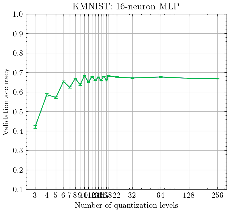
Observation 1: Accuracy Oscillates With Quantization

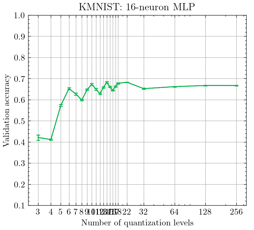
There appears to be an oscillation in accuracy when sweeping the number of quantization levels between 3 through 18. There are noticeable peaks at 6, 10, 14, and 18, and noticeable drops in accuracy at 8, 12, and 16 levels of quantization. What causes this oscillation?

The Hypothesis

I stared at the weights for a few hours and emerged with a hypothesis.

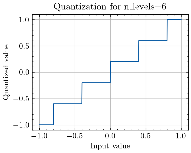
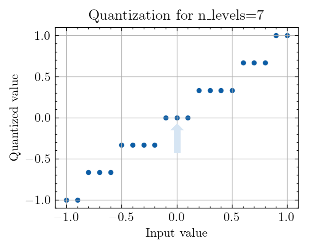
When the input image is quantized, the input pixels are only in range [0, 1], so this only uses half of the quantization levels, which are defined over the range [-1, 1]. In quantization schemes with even numbers of levels, the zero pixel values will either take on a small positive value, or a small negative value. Here’s what happens if you plot the quantized output as a function of floating point input. Nothing special to see here. There are exactly six steps.

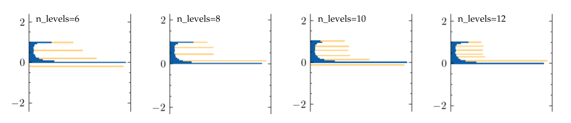
However, in cases where accuracy is low (8, 12, and 16 levels), the 0 pixel values get quantized to the positive side, and in cases where accuracy is high (6, 10, 14, 18), the zero pixel values get quantized to the nearest negative value. These plots plot histograms of the input pixel values $[0, 1]$ in blue, and their quantized values $[-1, 1]$ in orange. We see that for n_levels 6 and 10, the bottommost quantized value is less than 0, while for n_levels 8 and 12, the bottommost quantized value is greater than 0.

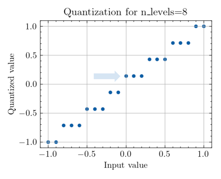
Going back to our quantization plot, the important question is, is the step open or closed at 0? Surprisingly, this changes between even numbers too:

When we take points at increments of 0.1, we see that actually 0 is mapped to -0.2, while anything slightly above 0 is mapped to 0.2.

And at an odd number of levels, the 0 value is mapped to exactly 0

With 8 levels, 0 is mapped to the step above 0

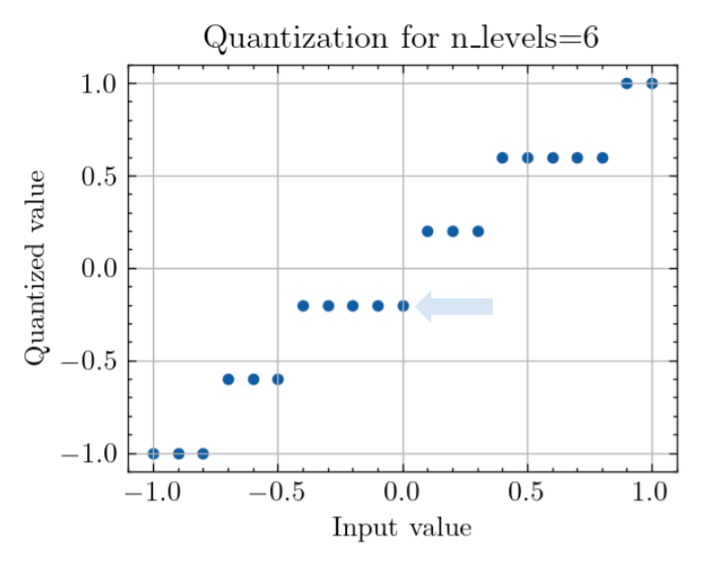
This oscillation seems to have a period of four, which aligns with what happens when you quantize the value of 0 at different quantization levels. The points where the quantized value is positive and far from 0 seem to correspond to the points where accuracy is significantly degraded (especially at 4 levels).

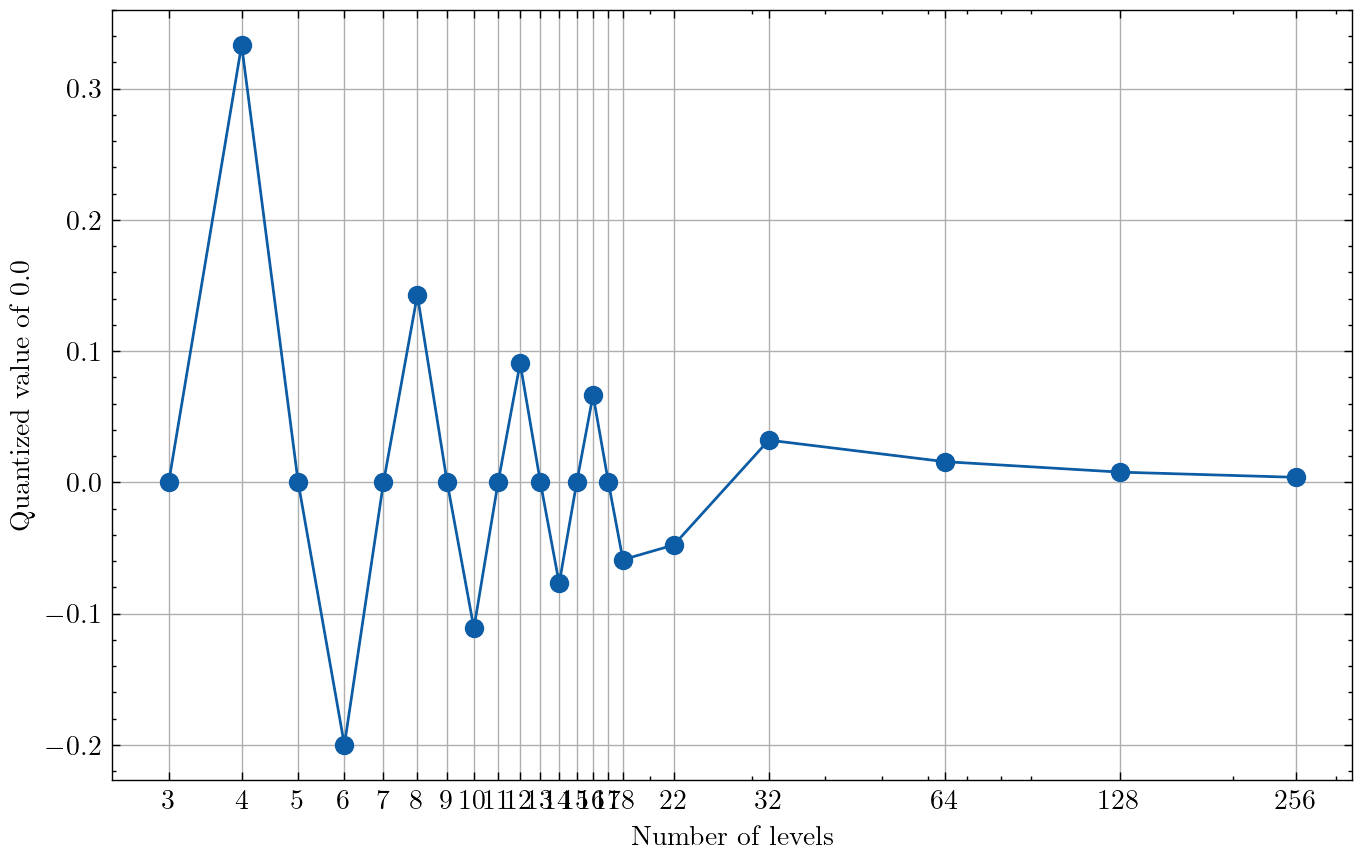
At a small number of levels of quantization, the zero pixel values are mapped farther away from 0 than with higher numbers of levels, which might be why this effect is most pronounced on the left side of the graph.

The Experiment

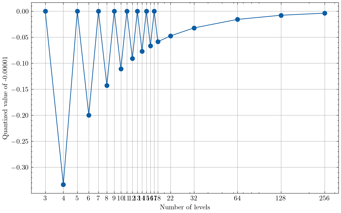
What if we took every pixel value that was 0, and instead replaced it with a pixel value that is -0.0001? This would be enough for the quantization function to always map those pixels to the level below 0 when the number of levels is even. In cases with an odd number of levels of quantization, this will not matter, and the -0.0001 value will still be quantized to 0. So we should expect either the values to be negative, or zero. If we do this, we see that as the number of levels of quantization increases, the “black” pixel value gets mapped to a value closer and closer to 0.

If we do this and re-run our sweep over the number of levels, we see that the oscillations with period 4 completely disappear!⊕Why might mapping pixel values of 0 to the next positive level perform worse than mapping pixel values of 0 to the next negative level? A feasible answer is that by quantizing upwards, black pixel values get lumped together with dark gray pixel values, while when quantizing downwards, black pixel values get their own level. If distinguishing between the dark colors of KMNIST is important, then quantizing to the negative value would perform much better. Which brings us to:

Observation 2: A Different Type of Oscillation

We seem to have fixed one problem: 4, 8, 12, and 16 previously had worse accuracy than their neighbors. But now, these networks have better accuracy than their neighbors!

This seems to be a new problem: there’s a new oscillation, with period 2! Furthermore, we might have expected that the odd-numbered constellations would perform better because the zero point value is mapped exactly to 0, while the even-numbered constellations introduce quantization noise. But here, it is the even-numbered constellations that do better than the odd-numbered constellations!

The Hypothesis

Clearly, the mapping of input values onto quantization levels has a significant effect on accuracy. What if we let the neural network choose the best mapping of input pixels to quantized values? This would let us see if the network preferred to map the 0 pixel value to the slightly positive or the slightly negative pixel value — or to something completely different altogether.

The Experiment

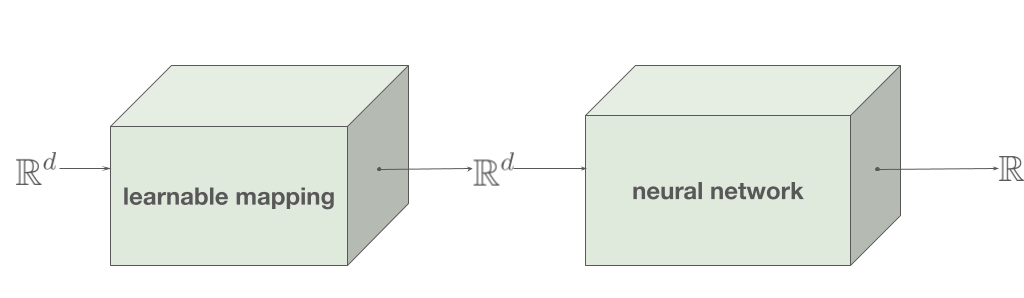
We can do this by adding an embedding: a map from input pixel values to values that go into the quantization function. This can be implemented by a Keras embedding layer, from a vector space (vocabulary) of dimension 1 to an embedding dimension also of dimension 1. The embedding is initialized to the identity function.

After training one instance of this network for 100 epochs, the mapping layer has learned a mapping that looks like this. Notice how the smallest pixel values are mapped to less than -0.5, while the second smallest set of values are mapped to 0. Post-quantization, the mapped points are in orange:

Learned mapping after using Adam optimizer to optimize embedding layer

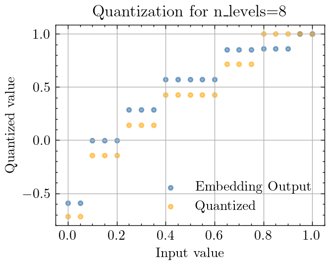
Learned mapping after using SGD to optimize embedding layer⊕These mappings demonstrate a strong preference to giving more space between the dark pixel values than the light pixel values, suggesting that it’s more important to distinguish between black and dark gray pixel values, than between white and light gray. This also aligns with our intuition for why mapping 0 pixel values downwards performs better than quantizing black pixels and gray pixels to the same value.

Now, running the same sweep over levels of quantization, we see that the oscillatory behavior completely disappears, and the accuracy pretty much monotonically increases with the number of quantization levels! ✨

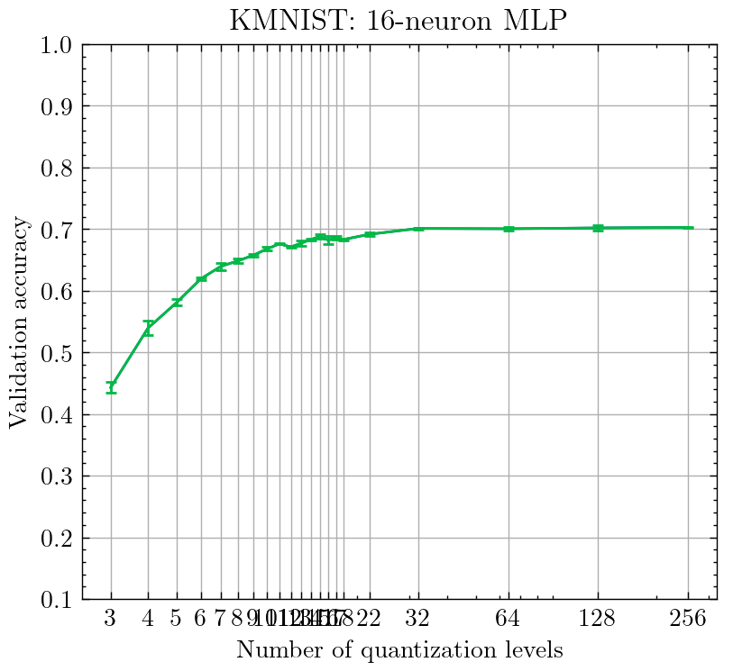
Furthermore, this scheme attains the highest accuracy compared to all the previous schemes, with the ceiling of accuracy at 70% compared to the previous 67-68%.

Observation 3: Distribution of Weights after Quantization-Aware Training

So we’ve been able to get to the smooth accuracy response to quantization that we’ve been seeking all along. But after staring at the weights a bit more, another strange pattern emerges.

We might assume that quantization-aware training produces weights that optimally make use of the quantized values. If we were to plot the distribution of the pre-quantization (full precision) weights, we might expect that the majority of weights cluster around the possible quantized values. However, we instead see the exact opposite:

Histogram of frequency of post-training weight values with 8-level quantization. On the x axis is the weight value between -1 and 1, and on the y axis is the frequency. The blue weights in full precision are quantized to the orange values during the forward pass.

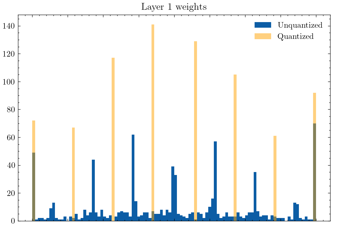
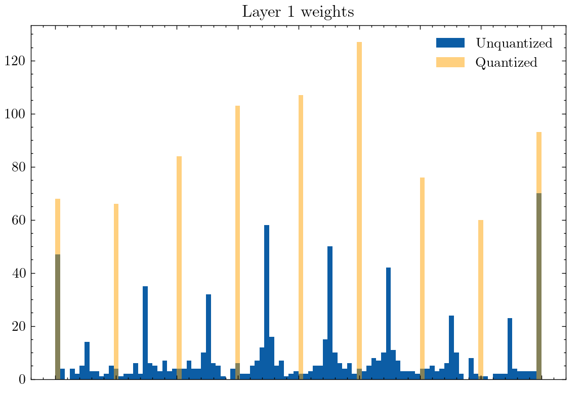
Surprisingly, for even-numbered levels of quantization (above with 8 levels), the weights actually take on values at the midpoint between the quantized levels. One might attribute this to the network wanting to represent a 0-point value, and there not being a 0 value post-quantization. So what if we give the network an odd number of levels in quantization (below: 9 levels)?

Histogram of frequency of post-training weight values with 9-level quantization. On the x axis is the weight value between -1 and 1, and on the y axis is the frequency. The blue weights in full precision are quantized to the orange values during the forward pass.

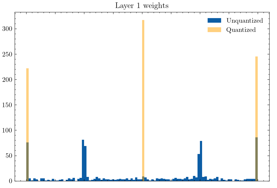
This behavior even exists at 3 levels of quantization:

Histogram of frequency of post-training weight values with 3-level quantization. On the x axis is the weight value between -1 and 1, and on the y axis is the frequency. The blue weights in full precision are quantized to the orange values during the forward pass.

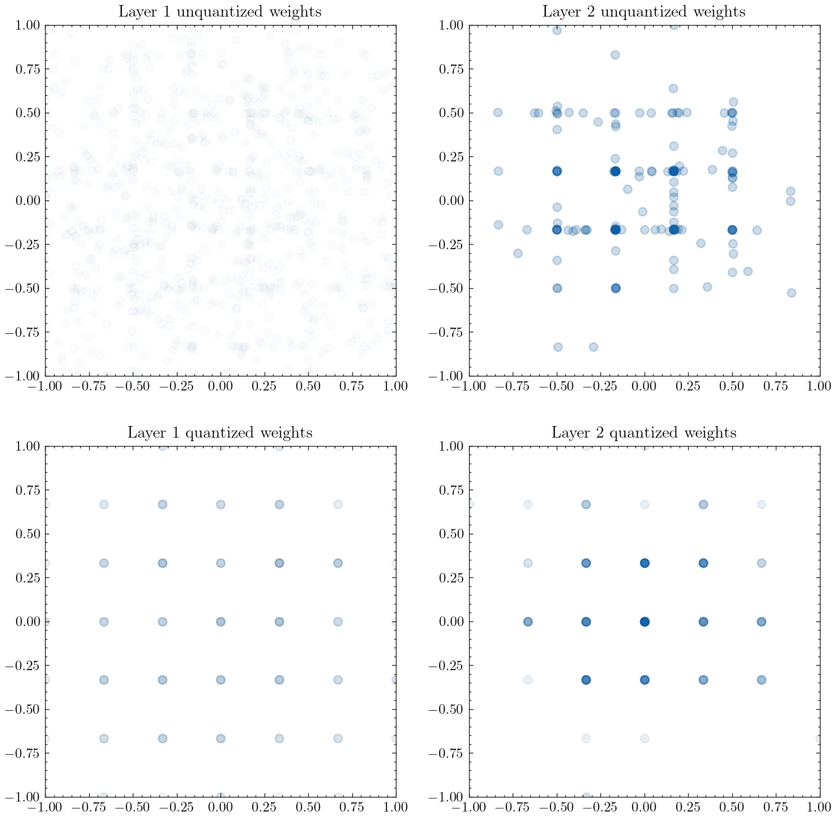
And this phenomenon even occurs in complex-valued neural networks, where most visibly in the Layer 2 weights, the unquantized weights cluster to points between two quantized weight values.

Heatmap of complex-valued weight values in a complex-valued neural network trained on the same KMNIST task. X and Y axes represent real and imaginary components of the weights.

Weights Oscillate During Training

We might understand this strange convergent behavior through the computation of gradients in quantization-aware training. Consider the case where we have a weight $w$ whose optimal value is between two levels of quantization. For the sake of example let’s look at the case of the 3-level quantization scheme above, and examine the range $[-1, 0]$.

Here, $w$ represents a full precision weight, while $Q(w)$ represents its quantized value. When the gradient update to $w$ is computed, the gradient is computed based on the full precision weight $Q(w)$. If $w$ is on one side of the midpoint, the gradient update will be much larger than the true value, because it will be computed based on $Q(w)$. This will push it over the midpoint, such that on the next update the gradient update will be computed based on the other $Q(w)$. This means that the full precision weight $w$ will bounce back and forth over the midpoint, and as the step size of each update decreases (as in the case of the Adam optimizer), the value of $w$ will converge to the exact midpoint between two neighboring quantization points.

In this process it is really rare for a weight to converge to exactly one of the quantized values, as the computation of the gradient using the quantized weights always gives a larger weight update than is really needed.  Even if the true gradient of $w$ is away from the center point, the usage of $ΔQ(w)$ as $Δw$ means the update to $w$ is in the wrong direction.

What’s next?

Weight oscillation during training is a known phenomenon with quantization-aware training, and was first pointed out in the 2022 paper “Overcoming Oscillations in Quantization-Aware Training”. They showed that existing QAT techniques don’t do much to solve these oscillations, and they propose oscillation dampening and iterative weight freezing as solutions.

While this is a simple model that lacks the complexity of digital QAT, we can still observe some of the same phenomena as digital QAT. This suggests the opportunity to apply learnings in digital quantization to enhance performance of analog quantized neural networks.⊕Shoutout to Frederic Jorgensen for the great discussion on weight oscillation!